Fetching data from CO-OPS SOS with Python tools¶

Pyoos is a high level data collection library for met/ocean data publicly available through many different websites and webservices.

In this post we will use pyoos to find and download data from the Center for Operational Oceanographic Products and Services (CO-OPS) using OGC’s SOS.

OGC: Open Geospatial Consortium
SOS: Sensor Observation Service

First we have to define a time span. Here we will fetch data during the hurricane Matthew passage over the southeast states from 2016-10-05 to 2016-10-12.

from datetime import datetime, timedelta

event_date = datetime(2016, 10, 9)

start_time = event_date - timedelta(days=4)
end_time = event_date + timedelta(days=3)

The geographical bounding box includes all the states in the SECOORA region: Florida, Georgia, South and North Carolina.

The variable of choice is sea level and we will convert any elevation units to meters.

import cf_units

units = cf_units.Unit("meters")

bbox = [-87.40, 24.25, -74.70, 36.70]

sos_name = "water_surface_height_above_reference_datum"

In this example we will use only the CoopsSos, but it is worth mentioning that pyoos has other collectors like IOOS SWE, NcSOS, 52N, NERRS, NDBC, etc.

Pyoos’ usage is quite simple, all we have to do is:

create an instance of the collector we will use and,
feed the instance with the data for the collection.

from pyoos.collectors.coops.coops_sos import CoopsSos

collector = CoopsSos()

collector.set_bbox(bbox)
collector.end_time = end_time
collector.start_time = start_time
collector.variables = [sos_name]

Let’s check we we got with the search above.

ofrs = collector.server.offerings
title = collector.server.identification.title

print("Collector offerings")
print("{}: {} offerings".format(title, len(ofrs)))

Collector offerings
NOAA.NOS.CO-OPS SOS: 1188 offerings

OK… That is quite misleading. We did not find 1113 stations with that search.

That number is probably all the CO-OPS SOS stations available.

In order to find out what we really get from that search we need to download the data. In the next two cells we will use a custom function to go from the collector object to a list of observations and a pandas DataFrame with all the data.

(Check the code for collector2table for the implementation details.)

import pandas as pd
from ioos_tools.ioos import collector2table

config = dict(units=units, sos_name=sos_name,)

data = collector2table(
    collector=collector,
    config=config,
    col="water_surface_height_above_reference_datum (m)",
)

# Clean the table.
table = dict(
    station_name=[s._metadata.get("station_name") for s in data],
    station_code=[s._metadata.get("station_code") for s in data],
    sensor=[s._metadata.get("sensor") for s in data],
    lon=[s._metadata.get("lon") for s in data],
    lat=[s._metadata.get("lat") for s in data],
    depth=[s._metadata.get("depth") for s in data],
)

table = pd.DataFrame(table).set_index("station_name")

table

	depth	lat	lon	sensor	station_code
station_name
Duck, NC	None	36.1833	-75.7467	urn:ioos:sensor:NOAA.NOS.CO-OPS:8651370:A1	8651370
Oregon Inlet Marina, NC	None	35.7950	-75.5481	urn:ioos:sensor:NOAA.NOS.CO-OPS:8652587:A1	8652587
USCG Station Hatteras, NC	None	35.2086	-75.7042	urn:ioos:sensor:NOAA.NOS.CO-OPS:8654467:A1	8654467
Beaufort, NC	None	34.7200	-76.6700	urn:ioos:sensor:NOAA.NOS.CO-OPS:8656483:A1	8656483
Wilmington, NC	None	34.2275	-77.9536	urn:ioos:sensor:NOAA.NOS.CO-OPS:8658120:B1	8658120
Wrightsville Beach, NC	None	34.2133	-77.7867	urn:ioos:sensor:NOAA.NOS.CO-OPS:8658163:A1	8658163
Springmaid Pier, SC	None	33.6550	-78.9183	urn:ioos:sensor:NOAA.NOS.CO-OPS:8661070:Y1	8661070
Oyster Landing (N Inlet Estuary), SC	None	33.3517	-79.1867	urn:ioos:sensor:NOAA.NOS.CO-OPS:8662245:A1	8662245
Charleston, Cooper River Entrance, SC	None	32.7808	-79.9236	urn:ioos:sensor:NOAA.NOS.CO-OPS:8665530:A1	8665530
Fort Pulaski, GA	None	32.0367	-80.9017	urn:ioos:sensor:NOAA.NOS.CO-OPS:8670870:A1	8670870
Fernandina Beach, FL	None	30.6714	-81.4658	urn:ioos:sensor:NOAA.NOS.CO-OPS:8720030:Y1	8720030
Mayport (Bar Pilots Dock), FL	None	30.3982	-81.4279	urn:ioos:sensor:NOAA.NOS.CO-OPS:8720218:A1	8720218
Dames Point, FL	None	30.3872	-81.5592	urn:ioos:sensor:NOAA.NOS.CO-OPS:8720219:A1	8720219
Southbank Riverwalk, St Johns River, FL	None	30.3205	-81.6591	urn:ioos:sensor:NOAA.NOS.CO-OPS:8720226:B1	8720226
Racy Point, St Johns River, FL	None	29.8002	-81.5498	urn:ioos:sensor:NOAA.NOS.CO-OPS:8720625:A1	8720625
Trident Pier, Port Canaveral, FL	None	28.4158	-80.5931	urn:ioos:sensor:NOAA.NOS.CO-OPS:8721604:A1	8721604
Lake Worth Pier, Atlantic Ocean, FL	None	26.6128	-80.0342	urn:ioos:sensor:NOAA.NOS.CO-OPS:8722670:N1	8722670
Virginia Key, Biscayne Bay, FL	None	25.7317	-80.1617	urn:ioos:sensor:NOAA.NOS.CO-OPS:8723214:A1	8723214
Vaca Key, Florida Bay, FL	None	24.7110	-81.1065	urn:ioos:sensor:NOAA.NOS.CO-OPS:8723970:A1	8723970
Key West, FL	None	24.5557	-81.8079	urn:ioos:sensor:NOAA.NOS.CO-OPS:8724580:A1	8724580
Naples, Gulf of Mexico, FL	None	26.1317	-81.8075	urn:ioos:sensor:NOAA.NOS.CO-OPS:8725110:A1	8725110
Fort Myers, Caloosahatchee River, FL	None	26.6480	-81.8710	urn:ioos:sensor:NOAA.NOS.CO-OPS:8725520:B1	8725520
Port Manatee, FL	None	27.6383	-82.5625	urn:ioos:sensor:NOAA.NOS.CO-OPS:8726384:A1	8726384
St Petersburg, Tampa Bay, FL	None	27.7606	-82.6269	urn:ioos:sensor:NOAA.NOS.CO-OPS:8726520:Y1	8726520
Old Port Tampa, FL	None	27.8578	-82.5528	urn:ioos:sensor:NOAA.NOS.CO-OPS:8726607:A1	8726607
Mckay Bay Entrance, FL	None	27.9130	-82.4250	urn:ioos:sensor:NOAA.NOS.CO-OPS:8726667:A1	8726667
Clearwater Beach, FL	None	27.9783	-82.8317	urn:ioos:sensor:NOAA.NOS.CO-OPS:8726724:A1	8726724
Cedar Key, FL	None	29.1336	-83.0309	urn:ioos:sensor:NOAA.NOS.CO-OPS:8727520:A1	8727520
Apalachicola, FL	None	29.7244	-84.9806	urn:ioos:sensor:NOAA.NOS.CO-OPS:8728690:A1	8728690
Panama City, FL	None	30.1523	-85.7000	urn:ioos:sensor:NOAA.NOS.CO-OPS:8729108:A1	8729108
Panama City Beach, FL	None	30.2133	-85.8783	urn:ioos:sensor:NOAA.NOS.CO-OPS:8729210:A1	8729210
Pensacola, FL	None	30.4044	-87.2100	urn:ioos:sensor:NOAA.NOS.CO-OPS:8729840:A1	8729840

In the next cell we will re-sample all the observation from CO-OPS’ original frequency (6 minutes) to 15 minutes to reduce the amount of data and hopefully some of the noise too.

index = pd.date_range(
    start=start_time.replace(tzinfo=None),
    end=end_time.replace(tzinfo=None),
    freq="15min",
)

# Re-index and rename series.
observations = []
for series in data:
    _metadata = series._metadata
    series.index = series.index.tz_localize(None)
    obs = series.reindex(index=index, limit=1, method="nearest")
    obs._metadata = _metadata
    obs.name = _metadata["station_name"]
    observations.append(obs)

We can now check the station with the highest sea elevation.

%matplotlib inline

df = pd.DataFrame(observations).T

station = df.max(axis=0).idxmax()

ax = df[station].plot(figsize=(7, 2.25))
title = ax.set_title(station)

../../../_images/2016-10-12-fetching_data_14_0.png

Oops. That does not look right! The data are near-real time, so some QA/QC may be needed before we move forward.

We can filter spikes with a simple first difference rule.

(Check the code for first_difference for the implementation details.)

from ioos_tools.qaqc import first_difference

mask = df.apply(first_difference, args=(0.99,))

df = df[~mask].interpolate()

ax = df[station].plot(figsize=(7, 2.25))
title = ax.set_title(station)

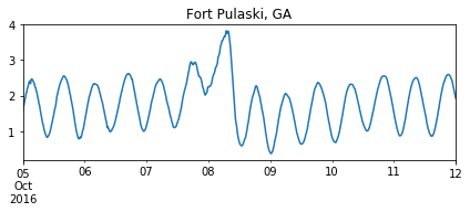
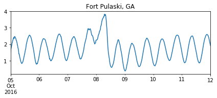
../../../_images/2016-10-12-fetching_data_16_0.png

That is much better! Now we can plot the station that actually registered the highest sea elevation.

station = df.max(axis=0).idxmax()

ax = df[station].plot(figsize=(7, 2.25))
title = ax.set_title(station)

../../../_images/2016-10-12-fetching_data_18_0.png

Let’s plot the last 5 stations, from North Carolina, so we can compare with Fort Pulaski, GA.

import matplotlib
import matplotlib.pyplot as plt

with matplotlib.style.context(["seaborn-notebook", "seaborn-darkgrid"]):
    fix, axes = plt.subplots(nrows=5, sharex=True, sharey=True, figsize=(11, 2.25 * 5))

    for k, obs in enumerate(observations[:5]):
        axes[k].plot(obs.index, obs.values)
        axes[k].text(obs.index[20], 0, obs._metadata["station_name"])

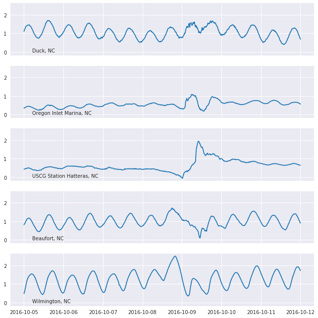
../../../_images/2016-10-12-fetching_data_20_0.png

Ideally we should filter out the tides in order to better interpret the storm surges. We’ll leave that as an exercise to the readers.

In order to easily explore all the stations we can put together an interactive map with the stations positions and the elevation time-series. This can be done using the software package bokeh and the mapping library folium.

from bokeh.embed import file_html
from bokeh.plotting import figure
from bokeh.resources import CDN
from folium import IFrame

# Plot defaults.
tools = "pan,box_zoom,reset"
width, height = 750, 250


def make_plot(series):
    p = figure(
        toolbar_location="above",
        x_axis_type="datetime",
        width=width,
        height=height,
        tools=tools,
        title=series.name,
    )
    line = p.line(
        x=series.index,
        y=series.values,
        line_width=5,
        line_cap="round",
        line_join="round",
    )
    return p, line


def make_marker(p, location, fname):
    html = file_html(p, CDN, fname)
    iframe = IFrame(html, width=width + 45, height=height + 80)

    popup = folium.Popup(iframe, max_width=2650)
    icon = folium.Icon(color="green", icon="stats")
    marker = folium.Marker(location=location, popup=popup, icon=icon)
    return marker

import folium

lon = (bbox[0] + bbox[2]) / 2
lat = (bbox[1] + bbox[3]) / 2

m = folium.Map(location=[lat, lon], tiles="OpenStreetMap", zoom_start=5)

for obs in observations:
    fname = obs._metadata["station_code"]
    location = obs._metadata["lat"], obs._metadata["lon"]
    p, _ = make_plot(obs)
    marker = make_marker(p, location=location, fname=fname)
    marker.add_to(m)

m

The U.S. Integrated Ocean Observing System (IOOS)

Fetching data from CO-OPS SOS with Python tools¶