Plotting Glider data with Python tools
In this notebook we demonstrate how to obtain and plot glider data using iris and cartopy. We will explore data from the Rutgers University RU29 Challenger glider that was launched from Ubatuba, Brazil on June 23, 2015 to travel across the Atlantic Ocean. After 282 days at sea, the Challenger was picked up off the coast of South Africa, on March 31, 2016. For more information on this ground breaking excusion see: https://marine.rutgers.edu/main/announcements/the-challenger-glider-mission-south-atlantic-mission-complete
Data collected from this glider mission are available on the IOOS Glider DAC THREDDS via OPeNDAP.
# See https://github.com/Unidata/netcdf-c/issues/1299 for the explanation of `#fillmismatch`.

url = (
    "https://data.ioos.us/thredds/dodsC/deployments/rutgers/"
    "ru29-20150623T1046/ru29-20150623T1046.nc3.nc#fillmismatch"
)
import iris

iris.FUTURE.netcdf_promote = True

glider = iris.load(url)

print(glider)
0: u Variable Quality Flag / (1)       (-- : 1; -- : 542; -- : 483)
1: precise_lon Variable Quality Flag / (1) (-- : 1; -- : 542; -- : 483)
2: longitude Variable Quality Flag / (1) (-- : 1; -- : 542; -- : 483)
3: Profile ID / (1)                    (-- : 1; -- : 542)
4: Platform Metadata / (1)             (-- : 1; -- : 542; -- : 483)
5: latitude Variable Quality Flag / (1) (-- : 1; -- : 542; -- : 483)
6: Trajectory Name / (1)               (-- : 1; -- : 64)
7: lon_uv Variable Quality Flag / (1)  (-- : 1; -- : 542; -- : 483)
8: v Variable Quality Flag / (1)       (-- : 1; -- : 542; -- : 483)
9: lat_uv Variable Quality Flag / (1)  (-- : 1; -- : 542; -- : 483)
10: precise_lat Variable Quality Flag / (1) (-- : 1; -- : 542; -- : 483)
11: WMO ID / (1)                        (-- : 1; -- : 64)
12: precise_time Variable Quality Flag / (1) (-- : 1; -- : 542; -- : 483)
13: time_uv Variable Quality Flag / (1) (-- : 1; -- : 542; -- : 483)
14: CTD Metadata / (1)                  (-- : 1; -- : 542; -- : 483)
15: eastward_sea_water_velocity / (m s-1) (-- : 1; -- : 542)
16: latitude / (degrees)                (-- : 1; -- : 542; -- : 483)
17: longitude / (degrees)               (-- : 1; -- : 542; -- : 483)
18: northward_sea_water_velocity / (m s-1) (-- : 1; -- : 542)
19: sea_water_density / (kg m-3)        (-- : 1; -- : 542; -- : 483)
20: sea_water_electrical_conductivity / (S m-1) (-- : 1; -- : 542; -- : 483)
21: sea_water_pressure / (dbar)         (-- : 1; -- : 542; -- : 483)
22: sea_water_salinity / (1e-3)         (-- : 1; -- : 542; -- : 483)
23: sea_water_temperature / (Celsius)   (-- : 1; -- : 542; -- : 483)
24: time / (seconds since 1970-01-01T00:00:00Z) (-- : 1; -- : 542; -- : 483)
/home/filipe/miniconda3/envs/IOOS/lib/python3.6/site-packages/iris/fileformats/cf.py:280: UserWarning: Missing CF-netCDF ancillary data variable 'lat_qc', referenced by netCDF variable 'precise_lat'
  warnings.warn(message % (name, nc_var_name))
/home/filipe/miniconda3/envs/IOOS/lib/python3.6/site-packages/iris/fileformats/cf.py:280: UserWarning: Missing CF-netCDF ancillary data variable 'lon_qc', referenced by netCDF variable 'precise_lon'
  warnings.warn(message % (name, nc_var_name))
Iris requires the data to adhere strictly to the CF-1.6 data model.
That is why we see all those warnings about Missing CF-netCDF ancillary data variable.
Note that if the data is not CF at all iris will refuse to load it!
The other hand, the advantage of following the CF-1.6 conventions,
is that the iris cube has the proper metadata is attached it.
We do not need to extract the coordinates or any other information separately .
All we need to do is to request the phenomena we want, in this case sea_water_density, sea_water_temperature and sea_water_salinity.
temp = glider.extract_strict("sea_water_temperature")
salt = glider.extract_strict("sea_water_salinity")
dens = glider.extract_strict("sea_water_density")

print(temp)
sea_water_temperature / (Celsius)   (-- : 1; -- : 542; -- : 483)
     Auxiliary coordinates:
          latitude                      x       x         -
          longitude                     x       x         -
          time                          x       x         -
          depth                         x       x         x
     Attributes:
          Conventions: Unidata Dataset Discovery v1.0, COARDS, CF-1.6
          DODS.dimName: wmo_id_strlen
          DODS.strlen: 7
          Easternmost_Easting: 13.5917595008
          Metadata_Conventions: Unidata Dataset Discovery v1.0, COARDS, CF-1.6
          Northernmost_Northing: -25.4926697853
          Southernmost_Northing: -37.3408904
          Westernmost_Easting: -44.9219533843
          _ChunkSizes: 1
          acknowledgment: This deployment supported by funding from the G.  Unger Vetelsen Foundation...
          actual_range: [  3.74399996  24.5387001 ]
          cdm_data_type: TrajectoryProfile
          cdm_profile_variables: time_uv,lat_uv,lon_uv,u,v,profile_id,time,latitude,longitude
          cdm_trajectory_variables: trajectory,wmo_id
          colorBarMaximum: 32.0
          colorBarMinimum: 0.0
          comment: Glider operatored by the Rutgers University Coastal Ocean Observation Lab,...
          contributor_name: Scott Glenn, Oscar Schofield, Josh Kohut, Antonio Ramos, Sebastian Swart,...
          contributor_role: Principal Investigator, Principal Investigator, Principal Investigator,...
          creator_email: kerfoot@marine.rutgers.edu
          creator_name: John Kerfoot
          creator_url: http://rucool.marine.rutgers.edu
          date_created: 2016-03-31T06:16:37Z
          date_issued: 2016-03-31T06:16:37Z
          featureType: TrajectoryProfile
          format_version: IOOS_Glider_NetCDF_v2.0.nc
          geospatial_lat_max: -25.4926697853
          geospatial_lat_min: -37.3408904
          geospatial_lat_units: degrees_north
          geospatial_lon_max: 13.5917595008
          geospatial_lon_min: -44.9219533843
          geospatial_lon_units: degrees_east
          geospatial_vertical_max: 983.17
          geospatial_vertical_min: 0.61
          geospatial_vertical_positive: down
          geospatial_vertical_units: m
          history: 2016-03-31T06:16:37Z /home/kerfoot/slocum/matlab/spt/export/nc/IOOS/DAC/writeIoosGliderFlatNc.m
2017-10-03T14:05:51Z...
          id: ru29-20150623T1046_f070_8f49_1646
          infoUrl: http://data.ioos.us/gliders/erddap/
          institution: Rutgers University
          instrument: instrument_ctd
          ioos_category: Temperature
          ioos_dac_checksum: fe452cc3a1bd121d6ba03cd41c4c004c
          ioos_dac_completed: True
          keywords: AUVS > Autonomous Underwater Vehicles, Oceans > Ocean Pressure > Water...
          keywords_vocabulary: GCMD Science Keywords
          license: This data may be redistributed and used without restriction.  Data provided...
          naming_authority: edu.rutgers.marine
          observation_type: measured
          platform: platform
          platform_type: Slocum Glider
          processing_level: Timestamp and gps positions checked for validity.
          project: Challenger
          publisher_email: kerfoot@marine.rutgers.edu
          publisher_name: John Kerfoot
          publisher_url: http://rucool.marine.rutgers.edu
          sea_name: South Atlantic Ocean
          source: Observational data from a profiling glider
          sourceUrl: (local files)
          standard_name_vocabulary: CF-v25
          subsetVariables: trajectory,wmo_id,time_uv,lat_uv,lon_uv,u,v,profile_id,time,latitude,l...
          summary: Third leg of the ru29 Challenger mission from Brazil to
            South...
          time_coverage_end: 2016-03-31T09:25:31Z
          time_coverage_start: 2015-06-23T10:57:59Z
          title: ru29-20150623T1046
          valid_max: 40.0
          valid_min: -5.0
Glider data is not something trivial to visualize. The very first thing to do is to plot the glider track to check its path.
import numpy.ma as ma

T = temp.data.squeeze()
S = salt.data.squeeze()
D = dens.data.squeeze()

x = temp.coord(axis="X").points.squeeze()
y = temp.coord(axis="Y").points.squeeze()
z = temp.coord(axis="Z")
t = temp.coord(axis="T")

vmin, vmax = z.attributes["actual_range"]

z = ma.masked_outside(z.points.squeeze(), vmin, vmax)
t = t.units.num2date(t.points.squeeze())

location = y.mean(), x.mean()  # Track center.
locations = list(zip(y, x))  # Track points.
import folium

tiles = (
    "http://services.arcgisonline.com/arcgis/rest/services/"
    "World_Topo_Map/MapServer/MapServer/tile/{z}/{y}/{x}"
)

m = folium.Map(location, tiles=tiles, attr="ESRI", zoom_start=4)

folium.CircleMarker(locations[0], fill_color="green", radius=10).add_to(m)
folium.CircleMarker(locations[-1], fill_color="red", radius=10).add_to(m)

line = folium.PolyLine(
    locations=locations,
    color="orange",
    weight=8,
    opacity=0.6,
    popup="Slocum Glider ru29 Deployed on 2015-06-23",
).add_to(m)

m
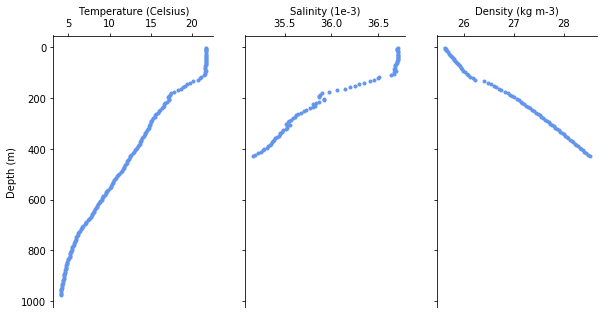
One might be interested in a the individual profiles of each dive. Lets extract the deepest dive and plot it.
import numpy as np

# Find the deepest profile.
idx = np.nonzero(~T[:, -1].mask)[0][0]
%matplotlib inline
import matplotlib.pyplot as plt

ncols = 3
fig, (ax0, ax1, ax2) = plt.subplots(
    sharey=True, sharex=False, ncols=ncols, figsize=(3.25 * ncols, 5)
)

kw = dict(linewidth=2, color="cornflowerblue", marker=".")
ax0.plot(T[idx], z[idx], **kw)
ax1.plot(S[idx], z[idx], **kw)
ax2.plot(D[idx] - 1000, z[idx], **kw)


def spines(ax):
    ax.spines["right"].set_color("none")
    ax.spines["bottom"].set_color("none")
    ax.xaxis.set_ticks_position("top")
    ax.yaxis.set_ticks_position("left")


[spines(ax) for ax in (ax0, ax1, ax2)]

ax0.set_ylabel("Depth (m)")
ax0.set_xlabel("Temperature ({})".format(temp.units))
ax0.xaxis.set_label_position("top")

ax1.set_xlabel("Salinity ({})".format(salt.units))
ax1.xaxis.set_label_position("top")

ax2.set_xlabel("Density ({})".format(dens.units))
ax2.xaxis.set_label_position("top")

ax0.invert_yaxis()
We can also visualize the whole track as a cross-section.
import numpy as np
import seawater as sw
from mpl_toolkits.axes_grid1.inset_locator import inset_axes


def distance(x, y, units="km"):
    dist, pha = sw.dist(x, y, units=units)
    return np.r_[0, np.cumsum(dist)]


def plot_glider(
    x, y, z, t, data, cmap=plt.cm.viridis, figsize=(9, 3.75), track_inset=False
):

    fig, ax = plt.subplots(figsize=figsize)
    dist = distance(x, y, units="km")
    z = np.abs(z)
    dist, z = np.broadcast_arrays(dist[..., np.newaxis], z)
    cs = ax.pcolor(dist, z, data, cmap=cmap, snap=True)
    kw = dict(orientation="vertical", extend="both", shrink=0.65)
    cbar = fig.colorbar(cs, **kw)

    if track_inset:
        axin = inset_axes(ax, width="25%", height="30%", loc=4)
        axin.plot(x, y, "k.")
        start, end = (x[0], y[0]), (x[-1], y[-1])
        kw = dict(marker="o", linestyle="none")
        axin.plot(*start, color="g", **kw)
        axin.plot(*end, color="r", **kw)
        axin.axis("off")

    ax.invert_yaxis()
    ax.set_xlabel("Distance (km)")
    ax.set_ylabel("Depth (m)")
    return fig, ax, cbar
from palettable import cmocean
haline = cmocean.sequential.Haline_20.mpl_colormap
thermal = cmocean.sequential.Thermal_20.mpl_colormap
dense = cmocean.sequential.Dense_20.mpl_colormap
fig, ax, cbar = plot_glider(x, y, z, t, S, cmap=haline, track_inset=False)
cbar.ax.set_xlabel("(g kg$^{-1}$)")
cbar.ax.xaxis.set_label_position("top")
ax.set_title("Salinity")
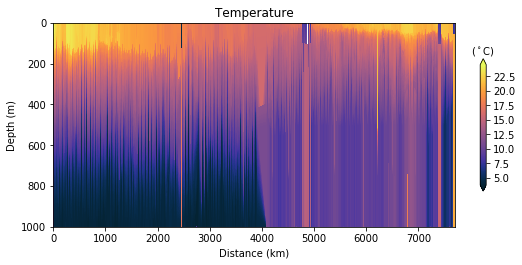
fig, ax, cbar = plot_glider(x, y, z, t, T, cmap=thermal, track_inset=False)
cbar.ax.set_xlabel(r"($^\circ$C)")
cbar.ax.xaxis.set_label_position("top")
ax.set_title("Temperature")
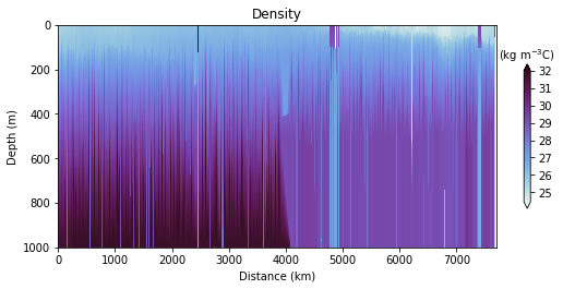
fig, ax, cbar = plot_glider(x, y, z, t, D - 1000, cmap=dense, track_inset=False)
cbar.ax.set_xlabel(r"(kg m$^{-3}$C)")
cbar.ax.xaxis.set_label_position("top")
ax.set_title("Density")
print("Data collected from {} to {}".format(t[0], t[-1]))
Data collected from 2015-06-23 10:57:59 to 2016-03-31 09:25:31
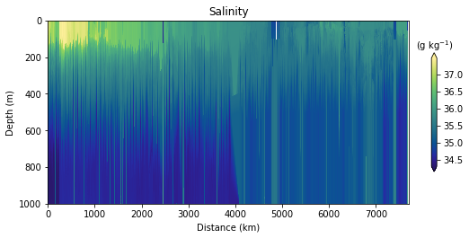
Glider cross-section also very be useful but we need to be careful when interpreting those due to the many turns the glider took, and the time it took to complete the track.
Note that the x-axis can be either time or distance. Note that this particular track took ~281 days to complete!
For those interested into more fancy ways to plot glider data check @lukecampbell’s profile_plots.py script.