Parsing Conventions and standards with Python
Metadata conventions, like the Climate and Forecast (CF) conventions, can be cumbersome to adhere to but it will be very handy when you or other users manipulate the data later in time.
In this notebook we will explore three Python modules that parse CF-1.6,
UGRID-1.0,
and SGRID-0.3
CF-1.6 with iris
There are many Python libraries to read and write CF metadata,
but only iris encapsulates CF in an object with an API.
From iris own docs:
Iris seeks to provide a powerful, easy to use, and community-driven Python library for analysing and visualising meteorological and oceanographic data sets.
With iris you can:
Use a single API to work on your data, irrespective of its original format.
Read and write (CF-)netCDF, GRIB, and PP files.
Easily produce graphs and maps via integration with matplotlib and cartopy.
import iris

iris.FUTURE.netcdf_promote = True

url = "http://tds.marine.rutgers.edu/thredds/dodsC/roms/espresso/2013_da/his/ESPRESSO_Real-Time_v2_History_fmrc.ncd"

cubes = iris.load(url)
/home/filipe/miniconda3/envs/IOOS/lib/python3.7/site-packages/iris/__init__.py:237: IrisDeprecation: setting the 'Future' property 'netcdf_promote' is deprecated and will be removed in a future release. Please remove code that sets this property.
  warn_deprecated(msg.format(name))
/home/filipe/miniconda3/envs/IOOS/lib/python3.7/site-packages/iris/fileformats/cf.py:1069: UserWarning: Ignoring formula terms variable 'zeta' referenced by data variable 'u' via variable 's_rho': Dimensions ('run', 'time', 'eta_rho', 'xi_rho') do not span ('run', 'time', 's_rho', 'eta_u', 'xi_u')
  warnings.warn(msg)
/home/filipe/miniconda3/envs/IOOS/lib/python3.7/site-packages/iris/fileformats/cf.py:1069: UserWarning: Ignoring formula terms variable 'h' referenced by data variable 'u' via variable 's_rho': Dimensions ('eta_rho', 'xi_rho') do not span ('run', 'time', 's_rho', 'eta_u', 'xi_u')
  warnings.warn(msg)
/home/filipe/miniconda3/envs/IOOS/lib/python3.7/site-packages/iris/fileformats/cf.py:1069: UserWarning: Ignoring formula terms variable 'zeta' referenced by data variable 'v' via variable 's_rho': Dimensions ('run', 'time', 'eta_rho', 'xi_rho') do not span ('run', 'time', 's_rho', 'eta_v', 'xi_v')
  warnings.warn(msg)
/home/filipe/miniconda3/envs/IOOS/lib/python3.7/site-packages/iris/fileformats/cf.py:1069: UserWarning: Ignoring formula terms variable 'h' referenced by data variable 'v' via variable 's_rho': Dimensions ('eta_rho', 'xi_rho') do not span ('run', 'time', 's_rho', 'eta_v', 'xi_v')
  warnings.warn(msg)
/home/filipe/miniconda3/envs/IOOS/lib/python3.7/site-packages/iris/fileformats/netcdf.py:599: UserWarning: Unable to find coordinate for variable 'zeta'
  '{!r}'.format(name))
/home/filipe/miniconda3/envs/IOOS/lib/python3.7/site-packages/iris/fileformats/netcdf.py:599: UserWarning: Unable to find coordinate for variable 'h'
  '{!r}'.format(name))
/home/filipe/miniconda3/envs/IOOS/lib/python3.7/site-packages/iris/fileformats/netcdf.py:719: UserWarning: Unable to construct Ocean s-coordinate, generic form 1 factory due to insufficient source coordinates.
  warnings.warn('{}'.format(e))
Aside: using iris.FUTURE.netcdf_promote = True we can promote netCDF formula terms,
like sea surface height, to first class cube objects.
This behavior will be default in future versions of iris and that line will not be needed after the next version of iris is released.
print(cubes)
0: S-coordinate bottom control parameter / (1) (scalar cube)
1: surface v-momentum stress / (newton meter-2) (forecast_reference_time: 1929; -- : 157; -- : 81; -- : 130)
2: number of time-steps between restart records / (1) (scalar cube)
3: tracers outflow, nudging inverse time scale / (second-1) (-- : 4; -- : 2)
4: tracers inflow, nudging inverse time scale / (second-1) (-- : 4; -- : 2)
5: 3D momentum nudging/relaxation inverse time scale / (day-1) (scalar cube)
6: constant Schmidt number for TKE / (1) (scalar cube)
7: surface u-momentum stress / (newton meter-2) (forecast_reference_time: 1929; -- : 157; -- : 82; -- : 129)
8: number of long time-steps / (1)     (scalar cube)
9: free-surface outflow, nudging inverse time scale / (second-1) (-- : 4)
10: surface flux from wave dissipation / (1) (scalar cube)
11: tracer point sources and sink activation switch / (1) (-- : 2)
12: mask on RHO-points / (1)            (-- : 82; -- : 130)
13: domain length in the ETA-direction / (meter) (scalar cube)
14: vertically integrated v-momentum component / (meter second-1) (forecast_reference_time: 1929; -- : 157; -- : 81; -- : 130)
15: starting time-step for accumulation of time-averaged fields / (1) (scalar cube)
16: nonlinear model Laplacian mixing coefficient for tracers / (meter2 second-1) (-- : 2)
17: 2D momentum inflow, nudging inverse time scale / (second-1) (-- : 4)
18: Coriolis parameter at RHO-points / (second-1) (-- : 82; -- : 130)
19: mask on psi-points / (1)            (-- : 81; -- : 129)
20: curvilinear coordinate metric in ETA / (meter-1) (-- : 82; -- : 130)
21: Power-law shape barotropic filter parameter / (1) (scalar cube)
22: quadratic drag coefficient / (1)    (scalar cube)
23: linear drag coefficient / (meter second-1) (scalar cube)
24: vertical momentum component / (meter second-1) (forecast_reference_time: 1929; -- : 157; ocean_s_coordinate_g1: 37; -- : 82; -- : 130)
25: number of time-steps between time-averaged records / (1) (scalar cube)
26: number of time-steps between history records / (1) (scalar cube)
27: 2D momentum nudging/relaxation inverse time scale / (day-1) (scalar cube)
28: turbulent length scale exponent / (1) (scalar cube)
29: number of time-steps between the creation of history files / (1) (scalar cube)
30: shear production coefficient / (1)  (scalar cube)
31: surface flux due to Craig and Banner wave breaking / (1) (scalar cube)
32: background vertical mixing coefficient for turbulent energy / (meter2 second-1) (scalar cube)
33: S-coordinate surface/bottom layer width / (meter) (scalar cube)
34: minimum value of specific turbulent kinetic energy / (1) (scalar cube)
35: 2D momentum outflow, nudging inverse time scale / (second-1) (-- : 4)
36: number of time-steps between the creation of average files / (1) (scalar cube)
37: stability coefficient / (1)         (scalar cube)
38: buoyancy production coefficient (plus) / (1) (scalar cube)
39: slipperiness parameter / (1)        (scalar cube)
40: time averaged v-flux for 3D equations coupling / (meter3 second-1) (forecast_reference_time: 1929; -- : 157; -- : 81; -- : 130)
41: NetCDF-4/HDF5 file format shuffle filer flag / (1) (scalar cube)
42: mask on U-points / (1)              (-- : 82; -- : 129)
43: Power-law shape barotropic filter parameter / (1) (scalar cube)
44: bottom roughness / (meter)          (scalar cube)
45: surface net heat flux / (watt meter-2) (forecast_reference_time: 1929; -- : 157; -- : 82; -- : 130)
46: bottom v-momentum stress / (newton meter-2) (forecast_reference_time: 1929; -- : 157; -- : 81; -- : 130)
47: surface roughness / (meter)         (scalar cube)
48: NetCDF-4/HDF5 file format deflate filer flag / (1) (scalar cube)
49: grid / (1)                          (scalar cube)
50: background vertical mixing coefficient for momentum / (meter2 second-1) (scalar cube)
51: background vertical mixing coefficient for length scale / (meter2 second-1) (scalar cube)
52: time averaged u-flux for 2D equations / (meter3 second-1) (forecast_reference_time: 1929; -- : 157; -- : 82; -- : 129)
53: 3D momentum outflow, nudging inverse time scale / (second-1) (-- : 4)
54: dissipation coefficient / (1)       (scalar cube)
55: stability exponent / (1)            (scalar cube)
56: constant Schmidt number for PSI / (1) (scalar cube)
57: background vertical mixing coefficient for tracers / (meter2 second-1) (-- : 2)
58: minimum Value of dissipation / (1)  (scalar cube)
59: Power-law shape barotropic filter parameter / (1) (scalar cube)
60: angle between XI-axis and EAST / (radians) (-- : 82; -- : 130)
61: grid type logical switch / (1)      (scalar cube)
62: vertical terrain-following transformation equation / (1) (scalar cube)
63: wave amplitude factor for surface roughness / (1) (scalar cube)
64: time stamp assigned to model initilization / (days since 2006-01-01 00:00:00) (scalar cube)
65: bottom u-momentum stress / (newton meter-2) (forecast_reference_time: 1929; -- : 157; -- : 82; -- : 129)
66: 3D momentum inflow, nudging inverse time scale / (second-1) (-- : 4)
67: vertically integrated u-momentum component / (meter second-1) (forecast_reference_time: 1929; -- : 157; -- : 82; -- : 129)
68: S-coordinate surface control parameter / (1) (scalar cube)
69: Tracers nudging/relaxation inverse time scale / (day-1) (-- : 2)
70: curvilinear coordinate metric in XI / (meter-1) (-- : 82; -- : 130)
71: mask on V-points / (1)              (-- : 81; -- : 130)
72: size of short time-steps / (second) (scalar cube)
73: time averaged u-flux for 3D equations coupling / (meter3 second-1) (forecast_reference_time: 1929; -- : 157; -- : 82; -- : 129)
74: nonlinear model Laplacian mixing coefficient for momentum / (meter2 second-1) (scalar cube)
75: NetCDF-4/HDF5 file format deflate level parameter / (1) (scalar cube)
76: mean density used in Boussinesq approximation / (kilogram meter-3) (scalar cube)
77: vertical terrain-following stretching function / (1) (scalar cube)
78: free-surface inflow, nudging inverse time scale / (second-1) (-- : 4)
79: turbulent kinetic energy exponent / (1) (scalar cube)
80: buoyancy production coefficient (minus) / (1) (scalar cube)
81: number of short time-steps / (1)    (scalar cube)
82: size of long time-steps / (second)  (scalar cube)
83: time averaged v-flux for 2D equations / (meter3 second-1) (forecast_reference_time: 1929; -- : 157; -- : 81; -- : 130)
84: domain length in the XI-direction / (meter) (scalar cube)
85: free-surface nudging/relaxation inverse time scale / (day-1) (scalar cube)
86: Charnok factor for surface roughness / (1) (scalar cube)
87: eastward_sea_water_velocity / (meter second-1) (forecast_reference_time: 1929; -- : 157; ocean_s_coordinate_g1: 36; -- : 82; -- : 129)
88: northward_sea_water_velocity / (meter second-1) (forecast_reference_time: 1929; -- : 157; ocean_s_coordinate_g1: 36; -- : 81; -- : 130)
89: sea_floor_depth / (meter)           (-- : 82; -- : 130)
90: sea_surface_height / (meter)        (forecast_reference_time: 1929; -- : 157; -- : 82; -- : 130)
91: sea_water_potential_temperature / (Celsius) (forecast_reference_time: 1929; -- : 157; ocean_s_coordinate_g1: 36; -- : 82; -- : 130)
92: sea_water_salinity / (1)            (forecast_reference_time: 1929; -- : 157; ocean_s_coordinate_g1: 36; -- : 82; -- : 130)
The advantages of the CF data model here are:
high level variable access via
standard_nameorlong_name;verbose warnings when there are compliance issues (see the units warnings above);
raise errors for non-compliant datasets;
separation of each phenomena (
variable) into its own cube*;each cube is a fully self-described format with all the original metadata;
round-trip load-save to netCDF is lossless;
free interpretation of the
formula_terms,cell_methods, andaxisthat helps with dimensionless coordinates, climatological variables, and plotting routines respectively.
* Most people miss the concept of a “dataset” when using iris,
but that is a consequence of the CF model.
Since there is no rule for unique names for the variables the dataset may contain the same phenomena with different coordinates,
hence iris decides to create an individual cube for each phenomena.
Aside: note that the xarray does have a dataset concept,
but it infringes the CF model in many places to do so.
We recommend xarray when CF compliance is not a requirement.
For more on iris see this example.
Moving on, let’s extract a single phenomena from the list of cubes above.
cube = cubes.extract_strict("sea_surface_height")

print(cube)
sea_surface_height / (meter)        (forecast_reference_time: 1929; -- : 157; -- : 82; -- : 130)
     Dimension coordinates:
          forecast_reference_time                           x          -         -        -
     Auxiliary coordinates:
          time                                              x          x         -        -
          latitude                                          -          -         x        x
          longitude                                         -          -         x        x
     Attributes:
          CPP_options: MyCPP, ADD_FSOBC, ADD_M2OBC, ANA_BSFLUX, ANA_BTFLUX, ASSUMED_SHAPE, AVERAGES,...
          Conventions: CF-1.4, SGRID-0.3
          DODS_EXTRA.Unlimited_Dimension: ocean_time
          EXTRA_DIMENSION.N: 36
          _ChunkSizes: [  1  82 130]
          _CoordSysBuilder: ucar.nc2.dataset.conv.CF1Convention
          ana_file: ROMS/Functionals/ana_btflux.h, /home/julia/ROMS/espresso/RealTime/Comp...
          avg_base: espresso_avg_4638
          bry_file: ../Data/espresso_bdry_new.nc
          cdm_data_type: GRID
          clm_file: ../Data/espresso_clm_new.nc
          code_dir: /home/julia/ROMS/espresso/svn1409
          compiler_command: /opt/pgisoft/openmpi/bin/mpif90
          compiler_flags:  -O3 -Mfree
          compiler_system: pgi
          cpu: x86_64
          featureType: GRID
          field: free-surface, scalar, series
          file: espresso_his_4638_0004.nc
          flt_file: espresso_flt_4638.nc
          format: netCDF-4/HDF5 file
          fpos_file: /home/om/cron/glider_floats/data/maracoos_floats.in
          frc_file_01: /home/om/roms/espresso/Data/espresso_tide_c05_20060101.nc
          frc_file_02: ../Data/espresso_river.nc
          frc_file_03: ../Data/rain_ncepnam_3hourly_MAB_and_GoM.nc
          frc_file_04: ../Data/swrad_ncepnam_3hourly_MAB_and_GoM.nc
          frc_file_05: ../Data/Tair_ncepnam_3hourly_MAB_and_GoM.nc
          frc_file_06: ../Data/Pair_ncepnam_3hourly_MAB_and_GoM.nc
          frc_file_07: ../Data/Qair_ncepnam_3hourly_MAB_and_GoM.nc
          frc_file_08: ../Data/lwrad_down_ncepnam_3hourly_MAB_and_GoM.nc
          frc_file_09: ../Data/Uwind_ncepnam_3hourly_MAB_and_GoM.nc
          frc_file_10: ../Data/Vwind_ncepnam_3hourly_MAB_and_GoM.nc
          grd_file: /home/om/roms/espresso/Data/espresso_grid_c05.nc
          header_dir: /home/julia/ROMS/espresso/RealTime/Compile/fwd
          header_file: espresso.h
          his_base: espresso_his_4638
          history: ROMS/TOMS, Version 3.5, Sunday - September 16, 2018 -  5:16:50 AM ;
FMRC...
          ini_file: /home/julia/ROMS/espresso/RealTime/Storage/run04/espresso_ini_4638.nc
          location: Proto fmrc:espresso_2013_da_his
          os: Linux
          rst_file: espresso_rst_4638.nc
          script_file: nl_ocean_espresso.in
          summary: Operational nowcast/forecast system version 2 for MARACOOS project (http://maracoos.org)....
          svn_rev: exported
          svn_url: https://www.myroms.org/svn/src/trunk
          tiling: 004x002
          time: ocean_time
          title: ROMS ESPRESSO Real-Time Operational IS4DVAR Forecast System Version 2 (NEW)...
          type: ROMS/TOMS history file
Requesting a vertical profile of temperature to see the formula_terms parsing in action.
(Note that ocean_s_coordinate_g1 is actually CF-1.7 but was backported to iris because it is widely adopted and the CF conventions document evolves quite slowly.)
temp = cubes.extract_strict("sea_water_potential_temperature")

print(temp)
sea_water_potential_temperature / (Celsius) (forecast_reference_time: 1929; -- : 157; ocean_s_coordinate_g1: 36; -- : 82; -- : 130)
     Dimension coordinates:
          forecast_reference_time                                   x          -                           -        -        -
          ocean_s_coordinate_g1                                     -          -                           x        -        -
     Auxiliary coordinates:
          time                                                      x          x                           -        -        -
          sea_surface_height                                        x          x                           -        x        x
          S-coordinate stretching curves at RHO-points              -          -                           x        -        -
          latitude                                                  -          -                           -        x        x
          longitude                                                 -          -                           -        x        x
          sea_floor_depth                                           -          -                           -        x        x
     Derived coordinates:
          sea_surface_height_above_reference_ellipsoid              x          x                           x        x        x
     Scalar coordinates:
          S-coordinate parameter, critical depth: 5.0 meter
     Attributes:
          CPP_options: MyCPP, ADD_FSOBC, ADD_M2OBC, ANA_BSFLUX, ANA_BTFLUX, ASSUMED_SHAPE, AVERAGES,...
          Conventions: CF-1.4, SGRID-0.3
          DODS_EXTRA.Unlimited_Dimension: ocean_time
          EXTRA_DIMENSION.N: 36
          _ChunkSizes: [  1  36  82 130]
          _CoordSysBuilder: ucar.nc2.dataset.conv.CF1Convention
          ana_file: ROMS/Functionals/ana_btflux.h, /home/julia/ROMS/espresso/RealTime/Comp...
          avg_base: espresso_avg_4638
          bry_file: ../Data/espresso_bdry_new.nc
          cdm_data_type: GRID
          clm_file: ../Data/espresso_clm_new.nc
          code_dir: /home/julia/ROMS/espresso/svn1409
          compiler_command: /opt/pgisoft/openmpi/bin/mpif90
          compiler_flags:  -O3 -Mfree
          compiler_system: pgi
          cpu: x86_64
          featureType: GRID
          field: temperature, scalar, series
          file: espresso_his_4638_0004.nc
          flt_file: espresso_flt_4638.nc
          format: netCDF-4/HDF5 file
          fpos_file: /home/om/cron/glider_floats/data/maracoos_floats.in
          frc_file_01: /home/om/roms/espresso/Data/espresso_tide_c05_20060101.nc
          frc_file_02: ../Data/espresso_river.nc
          frc_file_03: ../Data/rain_ncepnam_3hourly_MAB_and_GoM.nc
          frc_file_04: ../Data/swrad_ncepnam_3hourly_MAB_and_GoM.nc
          frc_file_05: ../Data/Tair_ncepnam_3hourly_MAB_and_GoM.nc
          frc_file_06: ../Data/Pair_ncepnam_3hourly_MAB_and_GoM.nc
          frc_file_07: ../Data/Qair_ncepnam_3hourly_MAB_and_GoM.nc
          frc_file_08: ../Data/lwrad_down_ncepnam_3hourly_MAB_and_GoM.nc
          frc_file_09: ../Data/Uwind_ncepnam_3hourly_MAB_and_GoM.nc
          frc_file_10: ../Data/Vwind_ncepnam_3hourly_MAB_and_GoM.nc
          grd_file: /home/om/roms/espresso/Data/espresso_grid_c05.nc
          header_dir: /home/julia/ROMS/espresso/RealTime/Compile/fwd
          header_file: espresso.h
          his_base: espresso_his_4638
          history: ROMS/TOMS, Version 3.5, Sunday - September 16, 2018 -  5:16:50 AM ;
FMRC...
          ini_file: /home/julia/ROMS/espresso/RealTime/Storage/run04/espresso_ini_4638.nc
          location: Proto fmrc:espresso_2013_da_his
          os: Linux
          rst_file: espresso_rst_4638.nc
          script_file: nl_ocean_espresso.in
          summary: Operational nowcast/forecast system version 2 for MARACOOS project (http://maracoos.org)....
          svn_rev: exported
          svn_url: https://www.myroms.org/svn/src/trunk
          tiling: 004x002
          time: ocean_time
          title: ROMS ESPRESSO Real-Time Operational IS4DVAR Forecast System Version 2 (NEW)...
          type: ROMS/TOMS history file
temp = cubes.extract_strict("sea_water_potential_temperature")

# Surface at the last time step.
T = temp[-1, -1, -1, ...]

# Random profile at the last time step.
t_profile = temp[-1, -1, :, 42, 42]
t_profile.coords(axis="Z")
[DimCoord(array([-0.98611111, -0.95833333, -0.93055556, -0.90277778, -0.875     ,
        -0.84722222, -0.81944444, -0.79166667, -0.76388889, -0.73611111,
        -0.70833333, -0.68055556, -0.65277778, -0.625     , -0.59722222,
        -0.56944444, -0.54166667, -0.51388889, -0.48611111, -0.45833333,
        -0.43055556, -0.40277778, -0.375     , -0.34722222, -0.31944444,
        -0.29166667, -0.26388889, -0.23611111, -0.20833333, -0.18055556,
        -0.15277778, -0.125     , -0.09722222, -0.06944444, -0.04166667,
        -0.01388889]), standard_name='ocean_s_coordinate_g1', units=Unit('1'), long_name='S-coordinate at RHO-points', var_name='s_rho', attributes={'_CoordinateAxes': 's_rho', '_CoordinateAxisType': 'GeoZ', '_CoordinateTransformType': 'Vertical', '_CoordinateZisPositive': 'up', 'field': 's_rho, scalar', 'positive': 'up', 'valid_max': 0.0, 'valid_min': -1.0}),
 AuxCoord(masked_array(data=[-27.951516510660785, -26.059303069671607,
                    -24.384124213287187, -22.89464875895186,
                    -21.562696436100815, -20.362612188354163,
                    -19.270701231552074, -18.264739397273928,
                    -17.3235917640554, -16.42699678498326,
                    -15.555599667979164, -14.691337378046954,
                    -13.818267733325536, -12.923866612931317,
                    -12.000663674133458, -11.047856433978302,
                    -10.072318055672692, -9.088358853495823,
                    -8.115873334297476, -7.1770917524024735,
                    -6.292781498350507, -5.479015518919441,
                    -4.7453534147148115, -4.094654850148295,
                    -3.5241580967286286, -3.027185090539729,
                    -2.594890101973965, -2.2176940552106283,
                    -1.8862775441376283, -1.5921597298211771,
                    -1.3279593376447076, -1.087444521211529,
                    -0.8654604836541105, -0.6577980350746284,
                    -0.46104300943631427, -0.2724290764393475],
              mask=[False, False, False, False, False, False, False, False,
                    False, False, False, False, False, False, False, False,
                    False, False, False, False, False, False, False, False,
                    False, False, False, False, False, False, False, False,
                    False, False, False, False],
        fill_value=1e+20), standard_name='sea_surface_height_above_reference_ellipsoid', units=Unit('meter'), attributes={'positive': 'up'})]
%matplotlib inline

import matplotlib.pyplot as plt
import numpy.ma as ma

T.data = ma.masked_invalid(T.data)

fig, ax = plt.subplots()

cs = ax.pcolormesh(T.data)
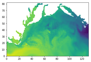
Iris knows about the metadata and can create fully annotated plots.
import iris.plot as qplt

qplt.plot(t_profile)
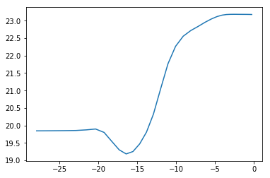
Be aware that too much automation may lead to some weird plots.
For example, the z-coord is in the x-direction and the automatic naming of the z to Sea surface height is above the reference ellipsoid in the second plot. Another example is the lack of proper coordinates in the first plot.
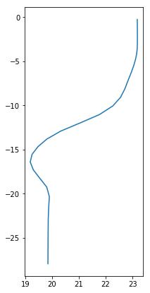
In these cases, manual plotting is more appropriate.
fig, ax = plt.subplots(figsize=(3, 7))

t = t_profile.data
z = t_profile.coord("sea_surface_height_above_reference_ellipsoid").points

ax.plot(t, z)
UGRID-1.0 with pyugrid
The Unstructured Grids convention encompasses any type of grid topology,
and the details of the convention are documented in https://ugrid-conventions.github.io/ugrid-conventions.
Right now pyugrid supports only triangular topologies, more will be added in the near future.
In a nutshell the pyugrid parses and exposes the underlying grid topology in a python object.
import pyugrid

url = "http://www.smast.umassd.edu:8080/thredds/dodsC/FVCOM/NECOFS/Forecasts/NECOFS_GOM3_FORECAST.nc"
ugrid = pyugrid.UGrid.from_ncfile(url)
Sometimes the topology is incomplete but,
if the data is UGRID compliant,
pyugrid can derive the rest for you.
ugrid.build_edges()
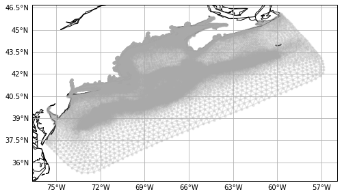
The topology can be extracted from ugrid object and used for plotting.
lon = ugrid.nodes[:, 0]
lat = ugrid.nodes[:, 1]
triangles = ugrid.faces[:]
import cartopy.crs as ccrs
from cartopy.mpl.gridliner import LATITUDE_FORMATTER, LONGITUDE_FORMATTER


def make_map(projection=ccrs.PlateCarree()):
    fig, ax = plt.subplots(figsize=(8, 6), subplot_kw=dict(projection=projection))
    ax.coastlines(resolution="50m")
    gl = ax.gridlines(draw_labels=True)
    gl.xlabels_top = gl.ylabels_right = False
    gl.xformatter = LONGITUDE_FORMATTER
    gl.yformatter = LATITUDE_FORMATTER
    return fig, ax


fig, ax = make_map()

kw = {"marker": ".", "linestyle": "-", "alpha": 0.25, "color": "darkgray"}
ax.triplot(lon, lat, triangles, **kw)
ax.coastlines()
There is some effort in the development community to integrate pyugrid into iris to augment the cube object to be both CF and UGRID aware.
It will add convenience plotting and slicing methods.
Check a longer pyugrid example here.
SGRID-0.3 with pysgrid
The Staggered Grid conventions help users to interpret grids from models like ROMS and DELFT, where the variables are defined in different grids. The specs are detailed in https://sgrid.github.io/sgrid.
The pysgrid module is similar to pyugrid. The grid topology is parsed into a Python object with methods and attributes that translate the SGRID conventions.
import pysgrid

url = "http://geoport.whoi.edu/thredds/dodsC/coawst_4/use/fmrc/coawst_4_use_best.ncd"
sgrid = pysgrid.load_grid(url)
All the raw grid information is present, like edges, dimensions, padding, grid center, and slicing.
sgrid.edge1_coordinates, sgrid.edge1_dimensions, sgrid.edge1_padding
(('lon_u', 'lat_u'),
 'xi_u: xi_psi eta_u: eta_psi (padding: both)',
 [GridPadding(mesh_topology_var='grid', face_dim='eta_u', node_dim='eta_psi', padding='both')])
u_var = sgrid.u

u_var.center_axis, u_var.node_axis
(1, 0)
v_var = sgrid.v
v_var.center_axis, v_var.node_axis
(0, 1)
u_var.center_slicing, v_var.center_slicing
((slice(None, None, None),
  slice(None, None, None),
  slice(1, -1, None),
  slice(None, None, None)),
 (slice(None, None, None),
  slice(None, None, None),
  slice(None, None, None),
  slice(1, -1, None)))
The API is “raw” but comprehensive. There is plenty of room to create convenience methods using the low level access provided by the library.
See below an example of the API and some simple convenience methods to slice, pad, average, and rotate the structure grid for plotting.
from netCDF4 import Dataset

# Compute the speed.
# **Rotate the grid.
# Average at the center.
from pysgrid.processing_2d import avg_to_cell_center, rotate_vectors, vector_sum

nc = Dataset(url)
u_velocity = nc.variables[u_var.variable]
v_velocity = nc.variables[v_var.variable]

v_idx = 0  # surface
time_idx = -1  # Last time step.

u = u_velocity[time_idx, v_idx, u_var.center_slicing[-2], u_var.center_slicing[-1]]
v = v_velocity[time_idx, v_idx, v_var.center_slicing[-2], v_var.center_slicing[-1]]


u = avg_to_cell_center(u, u_var.center_axis)
v = avg_to_cell_center(v, v_var.center_axis)


angles = nc.variables[sgrid.angle.variable][sgrid.angle.center_slicing]
u, v = rotate_vectors(u, v, angles)


speed = vector_sum(u, v)
** CF convention does describe the angle variable for grids that needs rotation, but there is no action expected. For example, in the formula_terms, pysgrid must be improved to abstract that action when needed via a simpler method.
<entry id="angle_of_rotation_from_east_to_x">
    <canonical_units>degree</canonical_units>
    <grib></grib>
    <amip></amip>
    <description>The quantity with standard name angle_of_rotation_from_east_to_x is the angle, anticlockwise reckoned positive, between due East and (dr/di)jk, where r(i,j,k) is the vector 3D position of the point with coordinate indices (i,j,k).  It could be used for rotating vector fields between model space and latitude-longitude space.</description>
</entry>
lon_var_name, lat_var_name = sgrid.face_coordinates

sg_lon = getattr(sgrid, lon_var_name)
sg_lat = getattr(sgrid, lat_var_name)

lon = sgrid.center_lon[sg_lon.center_slicing]
lat = sgrid.center_lat[sg_lat.center_slicing]
Ideally all the steps above could be performed in the background, in a high level object method call, like the iris cube plotting methods.
Let’s subset and center the velocity for better visualization (not a mandatory step but recommended).
def is_monotonically_increasing(arr, axis=0):
    return np.all(np.diff(arr, axis=axis) > 0)


def is_monotonically_decreasing(arr, axis=0):
    return np.all(np.diff(arr, axis=axis) < 0)


def is_monotonic(arr):
    return is_monotonically_increasing(arr) or is_monotonically_decreasing(arr)


def extent_bounds(arr, bound_position=0.5, axis=0):
    if not is_monotonic(arr):
        msg = "Array {!r} must be monotonic to guess bounds".format
        raise ValueError(msg(arr))

    x = arr.copy()
    x = np.c_[x[:, 0], (bound_position * (x[:, :-1] + x[:, 1:])), x[:, -1]]
    x = np.r_[
        x[0, :][None, ...],
        (bound_position * (x[:-1, :] + x[1:, :])),
        x[-1, :][None, ...],
    ]

    return x
import numpy as np

# For plotting reasons we will subsample every 10th point here
# 100 times less data!
sub = 10

lon = lon[::sub, ::sub]
lat = lat[::sub, ::sub]
u, v = u[::sub, ::sub], v[::sub, ::sub]
speed = speed[::sub, ::sub]

x = extent_bounds(lon)
y = extent_bounds(lat)
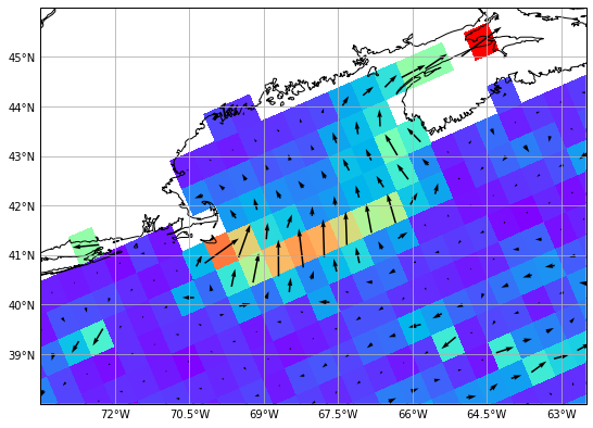
Now we can use quiver to plot the velocity components in a single grid.
def make_map(projection=ccrs.PlateCarree(), figsize=(9, 9)):
    fig, ax = plt.subplots(figsize=figsize, subplot_kw=dict(projection=projection))
    gl = ax.gridlines(draw_labels=True)
    gl.xlabels_top = gl.ylabels_right = False
    gl.xformatter = LONGITUDE_FORMATTER
    gl.yformatter = LATITUDE_FORMATTER
    return fig, ax
scale = 0.06

fig, ax = make_map()

kw = dict(scale=1.0 / scale, pivot="middle", width=0.003, color="black")
q = plt.quiver(lon, lat, u, v, zorder=2, **kw)

plt.pcolormesh(x, y, speed, zorder=1, cmap=plt.cm.rainbow)

c = ax.coastlines("10m")
ax.set_extent([-73.5, -62.5, 38, 46])
For more examples on pysgrid check this post out.