IOOS QARTOD software (ioos_qc)
This post will demonstrate how to run ioos_qc on a time-series dataset. ioos_qc implements the Quality Assurance / Quality Control of Real Time Oceanographic Data (QARTOD).
We will use bokeh for interactive plots, so let’s start by loading the interactive notebook output.
We will be using the water level data from a fixed station in Kotzebue, AK.
Below we create a simple Quality Assurance/Quality Control (QA/QC) configuration that will be used as input for ioos_qc. All the interval values are in the same units as the data.
For more information on the tests and recommended values for QA/QC check the documentation of each test and its inputs: https://ioos.github.io/ioos_qc/api/ioos_qc.html#module-ioos_qc.qartod
variable_name = "sea_surface_height_above_sea_level_geoid_mhhw"


qc_config = {
    "qartod": {
      "gross_range_test": {
        "fail_span": [-10, 10],
        "suspect_span": [-2, 3]
      },
      "flat_line_test": {
        "tolerance": 0.001,
        "suspect_threshold": 10800,
        "fail_threshold": 21600
      },
      "spike_test": {
        "suspect_threshold": 0.8,
        "fail_threshold": 3,
      }
    }
}
Now we are ready to load the data, run tests and plot results!
We will get the data from the AOOS ERDDAP server. Note that the data may change in the future. For reproducibility’s sake we will save the data downloaded into a CSV file.
from pathlib import Path
import pandas as pd
from erddapy import ERDDAP


path = Path().absolute()
fname = path.joinpath("data", "water_level_example.csv")

if fname.is_file():
    data = pd.read_csv(fname, parse_dates=["time (UTC)"])
else:
    e = ERDDAP(
        server="http://erddap.aoos.org/erddap/",
        protocol="tabledap"
    )
    e.dataset_id = "kotzebue-alaska-water-level"
    e.constraints = {
        "time>=": "2018-09-05T21:00:00Z",
        "time<=": "2019-07-10T19:00:00Z",
    }
    e.variables = [
        variable_name,
        "time",
        "z",
    ]
    data = e.to_pandas(
        index_col="time (UTC)",
        parse_dates=True,
    )
    data["timestamp"] = data.index.astype("int64") // 1e9
    data.to_csv(fname)

data.head()
| time (UTC) | sea_surface_height_above_sea_level_geoid_mhhw (m) | z (m) | timestamp | |
|---|---|---|---|---|
| 0 | 2018-09-05 21:00:00+00:00 | 0.4785 | 0.0 | 1.536181e+09 |
| 1 | 2018-09-05 22:00:00+00:00 | 0.4420 | 0.0 | 1.536185e+09 |
| 2 | 2018-09-05 23:00:00+00:00 | 0.4968 | 0.0 | 1.536188e+09 |
| 3 | 2018-09-06 01:00:00+00:00 | 0.5456 | 0.0 | 1.536196e+09 |
| 4 | 2018-09-06 02:00:00+00:00 | 0.5761 | 0.0 | 1.536199e+09 |
from ioos_qc.config import QcConfig


qc = QcConfig(qc_config)

qc_results =  qc.run(
    inp=data["sea_surface_height_above_sea_level_geoid_mhhw (m)"],
    tinp=data["timestamp"],
    zinp=data["z (m)"],
    gen_agg=True
)

qc_results
OrderedDict([('qartod',
              OrderedDict([('gross_range_test',
                            masked_array(data=[1, 1, 1, ..., 1, 1, 1],
                                         mask=False,
                                   fill_value=999999,
                                        dtype=uint8)),
                           ('flat_line_test', array([1, 1, 1, ..., 1, 1, 1])),
                           ('spike_test',
                            masked_array(data=[1, 1, 1, ..., 1, 1, 1],
                                         mask=False,
                                   fill_value=999999,
                                        dtype=uint8))]))])
The results are returned in a dictionary format, similar to the input configuration, with a mask for each test. While the mask is a masked array it should not be applied as such. The results range from 1 to 4 meaning:
data passed the QA/QC
did not run on this data point
flag as suspect
flag as failed
Now we can write a plotting function that will read these results and flag the data.
%matplotlib inline

from datetime import datetime

import numpy as np
import matplotlib.pyplot as plt


def plot_results(data, var_name, results, title, test_name):
    time = data["time (UTC)"]
    obs = data[var_name]
    qc_test = results["qartod"][test_name]

    qc_pass = np.ma.masked_where(qc_test != 1, obs)
    qc_suspect = np.ma.masked_where(qc_test != 3, obs)
    qc_fail = np.ma.masked_where(qc_test != 4, obs)
    qc_notrun = np.ma.masked_where(qc_test != 2, obs)

    fig, ax = plt.subplots(figsize=(15, 3.75))
    fig.set_title = f"{test_name}: {title}"

    ax.set_xlabel("Time")
    ax.set_ylabel("Observation Value")

    kw = {"marker": "o", "linestyle": "none"}
    ax.plot(time, obs,  label="obs", color="#A6CEE3")
    ax.plot(time, qc_notrun, markersize=2, label="qc not run", color="gray", alpha=0.2, **kw)
    ax.plot(time, qc_pass, markersize=4, label="qc pass", color="green", alpha=0.5, **kw)
    ax.plot(time, qc_suspect, markersize=4, label="qc suspect", color="orange", alpha=0.7, **kw)
    ax.plot(time, qc_fail, markersize=6, label="qc fail", color="red", alpha=1.0, **kw)
    ax.grid(True)


title = "Water Level [MHHW] [m] : Kotzebue, AK"
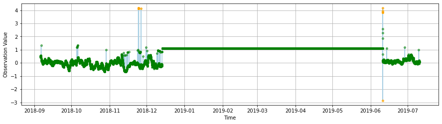
The gross range test test should fail data outside the \(\pm\) 10 range and suspect data below -2, and greater than 3. As one can easily see all the major spikes are flagged as expected.
plot_results(
    data,
    "sea_surface_height_above_sea_level_geoid_mhhw (m)",
    qc_results,
    title,
    "gross_range_test"
)
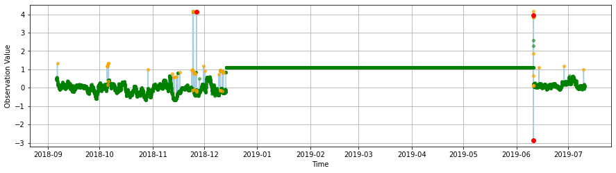
An actual spike test, based on a data increase threshold, flags similar spikes to the gross range test but also indetifies other suspect unusual increases in the series.
plot_results(
    data,
    "sea_surface_height_above_sea_level_geoid_mhhw (m)",
    qc_results,
    title,
    "spike_test"
)
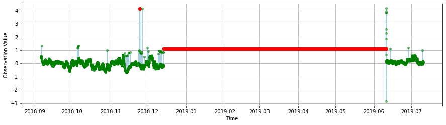
The flat line test identifies issues with the data where values are “stuck.”
ioos_qc succefully identified a huge portion of the data where that happens and flagged a smaller one as suspect. (Zoom in the red point to the left to see this one.)
plot_results(
    data,
    "sea_surface_height_above_sea_level_geoid_mhhw (m)",
    qc_results,
    title,
    "flat_line_test"
)
This notebook was adapt from Jessica Austin and Kyle Wilcox’s original ioos_qc examples. Please see the ioos_qc documentation for more examples.